Selecting Subsets of Data in Pandas: Part 3

Part 3: Assigning subsets of data

This is part three of a four-part series on how to select subsets of data from a pandas DataFrame or Series. Pandas offers a wide variety of options for subset selection which necessitates multiple articles. This series is broken down into the following topics.

1. Selection with [], .loc and .iloc
2. Boolean indexing
3. Assigning subsets of data
4. How NOT to select subsets of data

Become an Expert

If you want to be trusted to make decisions using pandas and scikit-learn, you must become an expert. I have completely mastered both libraries and have developed special techniques that will massively improve your ability and efficiency to do data analysis and machine learning.

• Master Data Analysis with Python — A comprehensive course with 600+ pages, 300+ exercises, multiple projects, and detailed solutions that will help you become a pandas expert.
• Master Machine Learning with Python — My comprehensive guide to become an expert at both the concepts and tools of building a machine learning workflow using Python with scikit-learn.
• Get a sample of the material by enrolling in the FREE Intro to Pandas course.
• Learn directly with me by taking an interactive and fun in-person bootcamp.

Assignment

When you see the word assign used during a discussion on programming, it usually means that a variable is set equal to some value. For most programming languages, this means using the equal sign. For instance, to assign the value 5 to the variable x in Python, we do the following:

>>> x = 5

This is formally called an assignment statement. More generally, we can define Python assignment statements as follows:

>>> variable = expression

There is quite a bit more to the Python assignment statement, but for our purposes it just means using the equal sign to store the object on the right-hand side to the left-hand side.

Social Media

I frequently post my python data science thoughts on social media. Follow me!

• Twitter @TedPetrou
• LinkedIn Ted Petrou
• Facebook Dunder Data

Corporate Training

If you have a group at your company looking to learn directly from an expert who understands how to teach and motivate students, let me know by filling out the form on this page.

Documentation on assigning subsets of data

There isn’t one particular sub-section of the documentation that covers this topic precisely. Several examples are available throughout the entire indexing section.

What does this have to do with selecting subsets of data?

In this article, we will use the assignment statement, but only after we select a subset of data. We will be doing our subset selection based on what we learned from part 1 and part 2 and changing just those values.

The left-hand side will have our subset selection and the right-hand side will contain our new values like this:

>>> subset_of_DataFrame_or_Series = new_values

Small sample dataset

During this tutorial, we will be working with a small sample of the employee dataset. The small dataset will help us immediately see the changes. Let’s take a look at this dataset now, which uses the index to store the names of each employee.

>>> import pandas as pd
>>> import numpy as np

>>> df = pd.read_csv('../../data/employee_sample.csv', index_col=0)
>>> df

 

 

Creating a new column

Before we change any of the data in this DataFrame, we will add a single column to the end. There are multiple ways of doing so, but we will begin by using just the indexing operator (the brackets). Place a string inside of the brackets and make this the left-hand side of the assignment.

The right-hand side can consist of any of the following:

• A scalar value
• A list or array with the same length as the DataFrame
• A pandas Series with an index that matches the index of the DataFrame (a little tricky!)

Master Data Analysis with Python

Master Data Analysis with Python is an extremely comprehensive course that will help you learn pandas to do data analysis.

I believe that it is the best possible resource available for learning how to data analysis with pandas and provide a 30-day 100% money back guarantee if you are not satisfied.

New column assigned to a scalar value

A scalar value is simply one single value, like an integer, string, boolean or date. When using a scalar for column assignment, each value in the column will be the same. Let’s create a column SCORE and assign it the value 99.

>>> df['SCORE'] = 99

Where’s the output?

In the previous two notebooks, we were only making column selections (no equal signs) resulting in output displayed directly into the notebook after executing the line of code. In the above, we made an assignment, which will not yield any output. We must use an extra line to display our data.

>>> df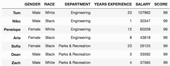

 

 

Create a new column with a list or array

Instead of creating a new column with all the same values, we can use a list or NumPy array with different values for each row. The only stipulation is that the number of new values in the list/array must be the same as the number of rows in the DataFrame.

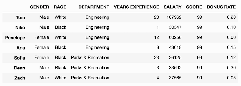
Let’s create the column BONUS RATE, with a list of numbers between 0 and 1.

>>> df['BONUS RATE'] = [.2, .1, 0, .15, .12, .3, .05]
>>> df

 

 

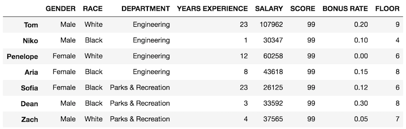
We could have just as easily used a one dimensional NumPy array to get the same exact results. Let’s do just that and create a random array of integers to represent the floor that the employee works on.

We use the randint function from NumPy's rand module. Use the low(inclusive) and high (exclusive) parameters to bound the range of possible integers. len(df) returns the number of rows in the DataFrame ensuring that the size of the array is correct.

>>> floor = np.random.randint(low=1, high=10, size=len(df))
>>> floor
array([9, 4, 6, 8, 6, 8, 7])

Then assign this to the FLOOR column:

>>> df['FLOOR'] = floor
>>> df

 

 

Creating a new column with a Series (tricky!)

Let’s create a new pandas Series and see what happens when we attempt to assign it as a new column in our DataFrame.

Let’s try and add a column for the last name of each person.

>>> last_name = pd.Series(['Smith', 'Jones', 'Williams', 'Green', 
                           'Brown', 'Simpson', 'Peters'])
>>> last_name
0       Smith
1       Jones
2    Williams
3       Green
4       Brown
5     Simpson
6      Peters
dtype: object

Make the assignment like we have done above:

>>> df['LAST NAME'] = last_name
>>> df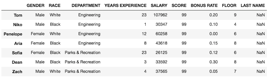

 

All missing values!

Our attempt failed because pandas uses a completely different methodology for combining two pandas objects.

Automatic alignment of the Index

Whenever two pandas objects are combined in some fashion the row/column index of one is aligned with the row/column index of the other. This all happens silently and implicitly behind the scenes. So if you are unaware of it, you will be completely taken by surprise. I will dedicate several notebooks in a different section to this surprising yet powerful feature.

Our operation failed to add the last names because the index of our Series is the integers 0 through 6, while the index of the DataFrame are the names of the employees. There are no index values in common between the objects, so pandas defaults to NaN (Not a number).

Create a Series with same Index as DataFrame

To use a Series to create a new column, the index must match that of the modifying DataFrame. Let’s re-create our Series with the same index as the DataFrame.

>>> last_name = pd.Series(data=['Smith', 'Jones', 'Williams', 
                                'Green', 'Brown', 'Simpson', 
                                'Peters'],
                      index=['Tom', 'Niko', 'Penelope', 'Aria', 
                             'Sofia', 'Dean', 'Zach'])
>>> last_name
Tom            Smith
Niko           Jones
Penelope    Williams
Aria           Green
Sofia          Brown
Dean         Simpson
Zach          Peters
dtype: object

Let’s try that assignment again. This technically will overwrite our previous LAST NAME column

>>> df['LAST NAME'] = last_name
>>> df

 

Create a new column with expressions involving other columns

We can create a new column by combining any number of other columns. One primary way of doing that is through a mathematical expression. For instance, let’s create a new column BONUS by multiplying the BONUS RATE andSALARY columns together.

Output before assignment

Before adding this new column to your DataFrame, you might want to consider viewing the output before making the assignment. This gives you a little preview so that you can check your work before doing the more permanent assignment.

Let’s multiple our two columns without assignment:

>>> df['BONUS RATE'] * df['SALARY']
Tom         21592.40
Niko         3034.70
Penelope        0.00
Aria         6542.70
Sofia        3135.00
Dean        10077.60
Zach         1878.25
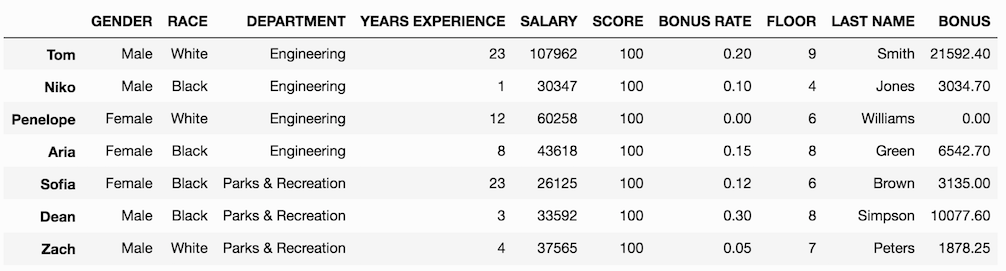
dtype: float64

Everything appears to be OK, so go ahead and make the assignment. Notice that the output is a Series with index the same as the DataFrame.

>>> df['BONUS'] = df['BONUS RATE'] * df['SALARY']
>>> df

 

 

Actual Subset Assignment

So far, we have just added new columns to our DataFrame. We did not change any of the pre-existing values. Let’s begin doing this by changing each person’s SCORE to 100.

The syntax is the same, whether it’s adding a new column or changing an existing column:

>>> df['SCORE'] = 100
>>> df

 

 

Overwriting the same column

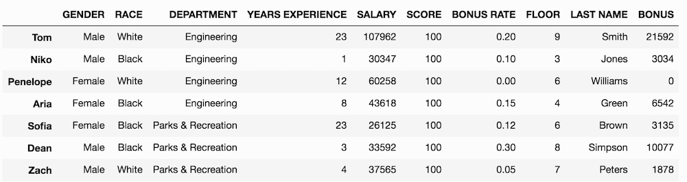
You can use the column itself you are assigning in the expression on the right-hand side of the equal sign. For instance, if we want to remove the ugly decimals from the BONUS column, we can call the astype method on it and assign it to itself.

>>> df['BONUS'] = df['BONUS'].astype(int)
>>> df

 

 

Assigning a subset of rows within a single column

Now that we can change all the values in a single column at once, let’s learn how to change just a subset of them.

For instance, let’s change the FLOOR for Niko, Penelope, and Aria. Before doing so, let's remember how to make that subset selection with .loc:

>>> df.loc[['Niko', 'Penelope', 'Aria'], 'FLOOR']
Niko        4
Penelope    6
Aria        8
Name: FLOOR, dtype: int64

The .loc indexer allows for row and column selection separated by a comma. It only makes selections based on row/column labels. Once we have correctly selected our subset, let's assign it a list of three new integers:

>>> df.loc[['Niko', 'Penelope', 'Aria'], 'FLOOR'] = [3, 6, 4]
>>> df

 

Style DataFrame to show differences (advanced)

It’s not important you understand this section if you are new to pandas, but you should still read through it as the style_diff function will be used in subsequent sections. Pandas provides a style attribute which allows you to apply a wide variety of CSS styles to your DataFrames. Check the style documentation for more.

We are going to change the background color and the color of the text for the values that have changed. To do this, you need to create a copy of the DataFrame before you make any changes with the copy method.

>>> df_orig = df.copy()

Then, we make our changes to our DataFrame

>>> df.loc[['Niko', 'Penelope', 'Aria'], 'FLOOR'] = [60, 42, 99]
>>> df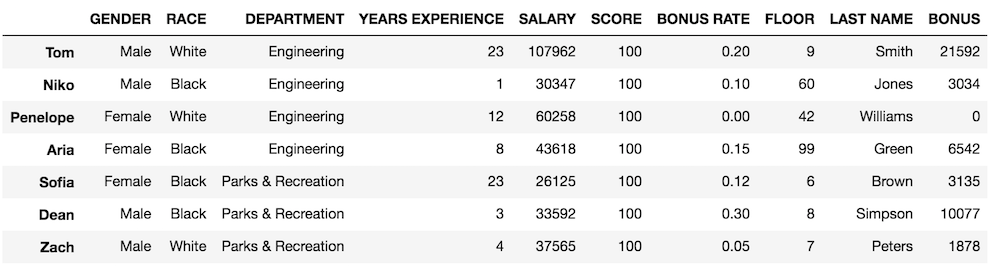

 

 

We can see that the values have changed, but it would be a bit nicer if they stood out more. The function below accepts both the new and original DataFrames. It then creates a boolean DataFrame and replaces all the Falsevalues with a semi-colon separated list of new CSS table attribute: valuepairs. The True values get replaced with empty strings. Pandas uses this DataFrame to know what style to apply to each cell.

>>> def style_diff(df, df_orig):
        style = {True: '', 
                 False: 'color: red; background-color: yellow'}
        df_style = (df == df_orig).replace(style)
        return df.style.apply(lambda x: df_style, axis=None)

We can use this function with any DataFrame that we have. But, take care when using a large DataFrame as the style DataFrames output every single row. So, if you have a 10,000 row DataFrame, you are probably going to crash your notebook.

>>> style_diff(df, df_orig)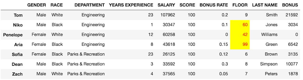

 

 

Assigning subsets with .iloc

Similarly, we can use the .iloc indexer which only makes selections via integer location.

Let’s assign the 3rd — 6th rows of the SCORE column (integer location 5) with the value 99. Again, we will make a copy of the DataFrame and display the difference with our style_diff function.

>>> df_orig = df.copy()
>>> df.iloc[3:6, 5] = 99
>>> style_diff(df, df_orig)

 

Assigning an entire column with .loc and .iloc

Normally, just the indexing operator is used to change values of an entire column, but it’s also possible to do it with both .loc and .iloc. You have to remember that the fist selection made by both these indexers is the rows. To select all rows, use the colon :.

For instance, let’s see this in action by changing all values in the FLOORcolumn.

>>> df_orig = df.copy()
>>> df.loc[:, 'FLOOR'] = 33
>>> style_diff(df, df_orig)

 

And with .iloc:

>>> df_orig = df.copy()
>>> df.iloc[:, 7] = 22
>>> style_diff(df, df_orig)

 

Assigning with boolean selection

It is more common to use boolean selection to make assignments to subsets than with directly selecting subsets by label or integer location.

For instance, let’s say we wanted to give everyone in the engineering department a $5,000 bonus on top of what they already have.

Before making the assignment, let’s properly select the data with boolean indexing.

>>> df.loc[df['DEPARTMENT'] == 'Engineering', 'BONUS']
Tom         21592
Niko         3034
Penelope        0
Aria         6542
Name: BONUS, dtype: int64

Once we have confirmed that our selection works, we can make an assignment. We can use the += operator to shorten the syntax considerably, which will assign the value back to itself.

>>> df_orig = df.copy()
>>> df.loc[df['DEPARTMENT'] == 'Engineering', 'BONUS'] += 5000
>>> style_diff(df, df_orig)

 

Assigning with multiple condition boolean selection

Let’s do an example with multiple boolean conditions. Let’s subtract 10 from the SCORE of all the black females and white males.

# check our logic first
>>> white_male = (df['GENDER'] == 'Male') & (df['RACE'] == 'White')
>>> black_female = ((df['GENDER'] == 'Female') & 
                    (df['RACE'] == 'Black'))
>>> criteria = white_male | black_female
>>> df[criteria]

 

>>> df_orig = df.copy()
>>> df.loc[criteria, 'SCORE'] -= 10
>>> style_diff(df, df_orig)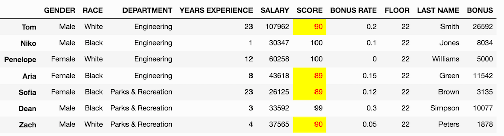

 

Assigning subsets of data in a Series

Assigning subsets of pandas Series is a less common operation but happens analogously to a DataFrame.

Let’s first select a copy of the SALARY column from our above DataFrame:

>>> s = df['SALARY'].copy()
>>> s
Tom         107962
Niko         30347
Penelope     60258
Aria         43618
Sofia        26125
Dean         33592
Zach         37565
Name: SALARY, dtype: int64

We didn’t have to use the copy method, but we did so to avoid theSettingWithCopy warning. This is a common warning when making assignments during subset selection. We will cover what it means and how to avoid it in the next notebook.

Assigning with .loc and .iloc

Since Series do not have columns, I don’t use just the indexing operator with them (unless I am doing boolean selection). It can be used to select rows, but is ambiguous and confusing and therefore I avoid it. All the capability of explicitly selecting particular Series values is provided with .loc and .iloc.

Let’s change the salary of Tom, Sofia, and Zach.

>>> s.loc[['Tom', 'Sofia', 'Zach']] = [99999, 39999, 49999]
>>> s
Tom         99999
Niko        30347
Penelope    60258
Aria        43618
Sofia       39999
Dean        33592
Zach        49999
Name: SALARY, dtype: int64

No styling with Series

Pandas outputs Series as plain text, so we cannot style them like we do with DataFrames.

However, we can create a function to modify the index by appending ‘-changed’ to the ones that have changed.

# advanced
>>> def style_diff_series(s, s_orig):
        idx = s.index.where(s == s_orig, s.index + '-changed')
        return s.set_axis(idx, inplace=False)

Create a copy of our original like we did before:

>>> s = df['SALARY'].copy()
>>> s_orig = s.copy()

Apply the changes:

>>> s.loc[['Tom', 'Sofia', 'Zach']] = [99999, 39999, 49999]

Add ‘changed’ to the index:

>>> style_diff_series(s, s_orig)
Tom-changed      99999
Niko             30347
Penelope         60258
Aria             43618
Sofia-changed    39999
Dean             33592
Zach-changed     49999
Name: SALARY, dtype: int64

We can make similar changes using integer location with .iloc. Here we change every other value.

>>> s_orig = s.copy()
>>> s.iloc[::2]  = 55555
>>> style_diff_series(s, s_orig)
Tom-changed         55555
Niko                30347
Penelope-changed    55555
Aria                43618
Sofia-changed       55555
Dean                33592
Zach-changed        55555
Name: SALARY, dtype: int64

Assigning Series with boolean indexing

We can use boolean indexing to make assignments as well. Using just the indexing operator is acceptable here. Let’s double all the salaries below 40,000.

>>> s_orig = s.copy()
>>> s[s < 40000] *= 2
>>> style_diff_series(s, s_orig)
Tom             55555
Niko-changed    60694
Penelope        55555
Aria            43618
Sofia           55555
Dean-changed    67184
Zach            55555
Name: SALARY, dtype: int64

Both just the indexing operator and .loc work the same when doing boolean indexing on a Series. However, as mentioned in part 2, .iloc should almost never be used when doing boolean indexing as it's not implemented fully.

Summary

• Assignment means using the equal sign to assign a variable on the left-hand side to an expression on the right-hand side
• New columns are created by passing a string to just the indexing operatorand setting it equal to either a scalar, a list/array the same length as the DataFrame, or a Series with an identical index as the DataFrame
• There is no output when you make an assignment. You must use an extra line to display the DataFrame/Series
• Select a specific subset of rows/columns with .loc or .iloc and manually assign them value with a list/array.
• Use the style attribute to make particular values pop out for visual display
• You can assign entire columns with .loc or .iloc by using the colon, :for rows
• A more common operation is to use boolean indexing to select subsets of data before making an assignment
• Assigning new values to a Series is similar to DataFrames except that we don’t use .iloc for boolean indexing

Just the basics of assignment of subsets

This tutorial covered the simplest and most frequently used assignment of subsets. The next notebook will cover some things NOT to do like chained indexing and triggering the SettingWithCopy warning.

There are also many other ways to create new columns or even add multiple columns at the same time. This notebook again is just drilling the basics.

Master Python, Data Science and Machine Learning

Immerse yourself in my comprehensive path for mastering data science and machine learning with Python. Purchase the All Access Pass to get lifetime access to all current and future courses. Some of the courses it contains:

• Master the Fundamentals of Python— A comprehensive introduction to Python (300+ pages, 150+ exercises)
• Master Data Analysis with Python — The most comprehensive course available to learn pandas. (800+ pages and 500+ exercises)
• Master Machine Learning with Python — A deep dive into doing machine learning with scikit-learn constantly updated to showcase the latest and greatest tools. (300+ pages)

Get the All Access Pass now!