Python for Data Analysis — A Critical Line-by-Line Review

In this post, I will offer my review of the book, Python for Data Analysis (2nd edition) by Wes McKinney. My name is Ted Petrou and I am an expert at pandas and author of the recently released Pandas Cookbook. I thoroughly read through PDA and created a very long, review that is available on github. This post provides some of the highlights from that full review.

What is a critical line-by-line review?

I read this book as if I was the only technical reviewer and I was counted on to find all the possible errors. Every single line of code was scrutinized and explored to see if a better solution existed. Having spent nearly every day of the last 18 months writing and talking about pandas, I have formed strong opinions about how it should be used. This critical examination lead to me finding fault with quite a large percentage of the code.

Begin Mastering Data Science Now for Free!

Take my free Intro to Pandas course to begin your journey mastering data analysis with Python.

Review Focuses on Pandas

The main focus of PDA is on the pandas library but it does have material on basic Python, IPython and NumPy, which are covered in chapters 1–4 and in the appendices. The pandas library is covered in chapters 5–14 and will be the primary focus of this review.

Overall Summary of PDA

PDA is similar to a Reference Manual

PDA is written very much like a reference manual, methodically covering one feature or operation before moving on to the next. The current version of the official documentation is a much more thorough reference guide if you are looking to learn pandas in a similar type of manner.

Little Data Analysis

There is very little actual data analysis and almost no teaching of common techniques or theory that are crucial to making sense of data.

Uses Randomly Generated Data

The vast majority of examples use randomly generated or contrived data that bear little resemblance to what data actually look like in the real world.

Operations are Learned in Isolation

For the most part, the operations are learned in isolation, independent from other parts of the pandas library. This is not how data analysis happens in the real world, where many commands from different sections of the library will be combined together to get a desired result.

Is Already Outdated

Although the commands will work for the current pandas version 0.21, it is clear that the book was not updated past version 0.18, which was released in March of 2016. This is apparent because the resample method gained the onparameter in version 0.19 which was absent in PDA. The powerful and popular function merge_asof was also added in version 0.19 and is not mentioned once in the book.

Lots of Non-Modern and Non-Idiomatic Code

There were numerous instances where it was clear that the book was not updated to show more modern code. For instance, the take method is almost never used any more and has been completely replaced by the .iloc indexer.There were also many instances where code snippets could be significantly transformed by using completely different syntax, which would result in much better performance and readability.

Indexing Confusion

One of the most confusing things for newcomers to pandas are the multiple ways to select data with the indexers[], .loc, and .iloc. There is not enough detailed explanations for the reader to walk away with a thorough understanding of each.

Chapter-by-Chapter Review

In this next section, I will give short summaries of each chapter followed by more details on specific code snippets.

Chapter 5. Getting Started with pandas

Chapter 5 covers an introduction to the primary pandas data structures, the Series and the DataFrame, and some of their more popular methods. The commands in this chapter can almost all be found directly in the pandas official documentation with greater depth. For instance, the book begins by producing a near replica of the intro section of the documentation. All of the index selection in the chapter is covered in greater detail in the indexing section of the documentation. Like most of the book, this chapter uses randomly generated or contrived data that has little application to real data analysis.

Chapter 5 Details

The book begins by erroneously stating that the Series and DataFrame constructors are used often. They are not, and most data is read directly into pandas as a DataFrame with the read_csv function or one of the many other functions that begin with read_. I would also not encourage people to import the constructors directly into their global namespace like this:

>>> from pandas import Series, DataFrame

Instead, it is more much more common to simply do: import pandas as pd.

Series and DataFrame Constructors
The first real line of code creates a Series with its consturctor. I don’t think Series and DataFrame construction should be covered first as it’s typically not used at all during most basic data analyses. PDA uses the variable name objto refer to the Series. I like to be more verbose and would refer to it as ser ors. DataFrames are given the better name frame but this is not typical of what is used throughout the pandas world. The documentation uses s for Series and df for DataFrames. On one occasion, the DataFrame is given the name data. Whatever name is used should be consistent.

Indexing
Data selection is covered next with the indexing operator, [] on a Series. This is a mistake. I highly discourage all pandas users to use the indexing operator by itself to select elements from a Series. It is ambiguous and not at all explicit. Instead, I advise always using .loc/.iloc to make selections from a Series. The only recommended use for the indexing operator is when doing boolean indexing.

For instance, PDA does:

>>> s = pd.Series(data=[9, -5, 13], index=['a', 'b', 'c'])
>>> s
a     9
b    -5
c    13
dtype: int64

# The indexing operator can take integers or labels and thus is ambiguous

>>> s[1]
-5

>>> s['b]
-5

When it should use .iloc for integers and .loc for labels:

>>> s.iloc[1]
-5

>>> s.loc['b']
5

apply method
I really don’t like teaching the apply method so soon as beginners almost always misuse it. There is almost always a better and more efficient alternative. In one of the cases, apply is used to aggregate by calling a custom function on each row. This is completely unnecessary, as there exists a quick and easy way to do it with the built-in pandas methods.

The data looks like this:

>>> df = pd.DataFrame(np.random.randn(4, 3), columns=list('abc'),
        index=['Quebec', 'Ontario', 'Alberta', 'Nova Scotia'])
>>> df

 

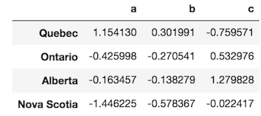
PDA then uses apply like this:

>>> df.apply(lambda x: x.max() - x.min())
a    2.600356
b    0.880358
c    2.039398
dtype: float64

A more idiomatic way to do this is with max and min methods directly:

>>> df.max() - df.min()
a    2.600356
b    0.880358
c    2.039398
dtype: float64

I understand that a contrived example is used here to understand the mechanics of apply, but this is exactly how new users get confused. apply is an iterative and slow method that should only be used if no other more efficient and vectorized solution exists. It is crucial to think of vectorized solutions not iterative ones. I see this mistake all the time when answering questions on Stack Overflow.

Another bad use of apply
There is another bad use of apply when a much simpler alternative exists with the agg method. Let’s create the data first:

>>> df = pd.DataFrame(np.random.randint(0, 10, (6,3)),  
                      columns=['Table', 'Chair', 'Bed'])
>>> df

 

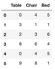
PDA finds the maximum and minimum value of each column like this:

>>> def f(x):
        return pd.Series([x.min(), x.max()], index=['min', 'max'])
        
>>> df.apply(f)

 

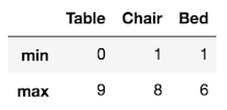
A much easier alternative exists with the agg method that produces the same exact output:

>>> df.agg(['min', 'max'])  

Chapter 6. Data Loading, Storage, and File Formats

Chapter 6 covers many of the ways to read data into a pandas DataFrame from a file. There are many functions that begin with read_ that can import nearly any kind of data format. Almost the entire chapter is covered in greater detail in the IO Tools section of the documentation. There is no actual data analysis in this chapter, just the mechanics of reading and writing files.

Chapter 6 Details

PDA fails to point out that read_csv and read_table are the same exact function except that read_csv defaults to a comma-separated delimiter andread_table defaults to tab-separated. There is absolutely no need for both of these functions and it’s confusing to go back and forth between them.

There is a section on iterating through a file with the csv module. PDA shows the mechanics of this with a file that actually needs no further processing. It could have been made much more interesting if there was some actual processing but there is none.

PDA covers the read_html function with nearly the exact same example from the documentation.

Chapter 7. Data Cleaning and Preparation

Chapter 7 follows the same pattern of using contrived and randomly generated data to show the basic mechanics of a few methods. It is devoid of actual data analysis and fails to show how to combine multiple pandas operations together. All of the methods in this chapter are covered in much greater detail in the documentation. Visit the Working with missing data section to get all the detailed mechanics of missing value manipulation in pandas. The chapter covers just a small amount of string manipulation. Visit the Working with the Text Data section to get more details.

This chapter contains a large amount of poor and inefficient pandas code. There is an extreme example of looping to fill a DataFrame that can be accomplished in much more concise code nearly 100x as fast.

Chapter 7 Details

The chapter begins by covering the isnull method, which is a little confusing because in Chapter 5, the function pd.isnull was used. I think a better job of distinguishing between methods and functions would be good here.

PDA continually uses axis=1 to refer to the columns in its method calls. I highly advise against doing this, as it is not as explicit and instead suggest the more explicit axis='columns'.

There should be a distinction between the map and apply methods. Ideally,map should only be used whenever you are passing a dictionary/Series to literally map one value to another. The apply method can only accept functions, so should always be used whenever you need to apply a function to your Series/DataFrame. Yes, map has the same ability to accept functions in a similar manner as apply, but this is why we need to have a separating boundary between the two methods. It helps to avoid confusion. In summary:

• Use map only when you want to literally map each value in a Series to another. Your mapping must be a dictionary or a Series
• Use apply when you have a function that you want to act on each individual member of the Series.
• Never pass a function to map

For instance, there is a Series with data like this:

>>> s = pd.Series(['Houston', 'Miami', 'Cleveland'])
>>> states_map = {'houston':'Texas', 'miami':'Florida',       
                  'Cleveland':'Ohio'}

PDA says to pass a function to the map method:

>>> s.map(lambda x: states_map[x.lower()])
0      Texas
1    Florida
2       Ohio
dtype: object

But if you are going to use a function, you should use apply in the same exact manner. It gives the same result and it has more options than map.

>>> s.apply(lambda x: states_map[x.lower()])

There is actually a simpler and more idiomatic way of doing this exercise. Generally, your mapping dictionary is going to be much smaller than the size of your Series. It makes more sense to conform the dictionary to the values in your Series. Here, we can simply change the keys in the dictionary (with thetitle string method) to match the values in our Series.

Let’s create a Series with 1 million elements and time the difference. This newer way is 6x as fast:

>>> s1 = s.sample(1000000, replace=True)

>>> %timeit s1.str.lower().map(states_map) # slow from PDA
427 ms ± 12.1 ms per loop (mean ± std. dev. of 7 runs, 1 loop each)

>>> %timeit s1.map({k.title(): v for k, v in states_map.items()})
73.6 ms ± 909 µs per loop (mean ± std. dev. of 7 runs, 10 loops each)

Detecting and Filtering Outliers
In this section, boolean indexing is used to find values in a Series that have absolute value greater than 3. PDA uses the NumPy function abs. NumPy functions should not be used when identical pandas methods are available:

>>> s = pd.Series(np.random.randn(1000))
>>> s[np.abs(s) > 3]  # Don't use numpy
>>> s[s.abs() > 3]    # Use pandas methods

A particularly bad piece of code in PDA caps the values in a DataFrame to be between -3 and 3 like this:

>>> data[np.abs(data) > 3] = np.sign(data) * 3

Pandas comes equipped with the clip method which simplifies things quite a bit:

>>> data.clip(-3, 3)

Permutation and Random Sampling
The take method is shown which is almost never used anymore. Its functionality was replaced by the .iloc indexer:

>>> sampler = [5, 2, 8, 10]
>>> df.take(sampler)  # outdated - don't use
>>> df.iloc[sampler]  # idiomatic

Computing Indicator/Dummy Variables
One of the most inefficient pieces of code in the entire books comes in this section. A DataFrame is constructed to show indicator columns (0/1) for each movie genre. The code creates an all zeros DataFrame then fills it with the rarely used get_indexer index method:

>>> zero_matrix = np.zeros((len(movies), len(genres)))
>>> dummies = pd.DataFrame(zero_matrix, columns=genres)

>>> for i, gen in enumerate(movies.genres):
        indices = dummies.columns.get_indexer(gen.split('|'))
        dummies.iloc[i, indices] = 1

>>> movies_windic = movies.join(dummies.add_prefix('Genre_'))
>>> movies_windic.head()

This code is incredibly slow and not idiomatic. The movies DataFrame is only 3,883 rows and takes a whopping 1.2 seconds to complete. There are several methods that are much faster.

An iterative approach would simply create a nested dictionary of dictionaries and pass this to the DataFrame constructor:

>>> d = {}
>>> for key, values in movies.genres.items():
        for v in values.split('|'):
            if v in d:
                d[v].update({key:1})
            else:
                d[v] = {key:1}       
>>> df = movies.join(pd.DataFrame(d).fillna(0))

This takes only 14 ms, about 85 times faster the approach used in PDA.

Chapter 8. Data Wrangling: Join, Combine, and Reshape

Chapter 8 is another chapter with fake data and covers very basic mechanics of many operations independently. There is very little code that combines multiple pandas methods together like is done in the real world. The hierarchical indexing is likely going to confuse readers as it is quite complex and suggest reading the documentation on hierarchical indexing.

The sections on merge and join don’t cover the differences between the two well-enough and the examples again are very dry. See the documentation on merging for more.

Chapter 8 Details

In one block of code, both the indexing operator, [], and .loc are used to select Series elements. This is confusing and as I’ve said multiple times, stick with using only .loc/.iloc except when doing boolean indexing.

Pivoting “Long” to “Wide” Format
Finally, we get to a more interesting situation. There needs to be a mention of tidy vs messy data here from the Hadley Wickham . The first dataset used is actually tidy and doesn’t need any reshaping at all. And when the data is reshaped into ‘long’ data, it actually becomes messy.

The reset_index method has the name parameter to rename the Series values when it becomes a column. There is no need for a separate call:

### Unecessary
>>> ldata = data.stack().reset_index().rename(columns={0: ‘value’})

### Can shorten to
>>> ldata = data.stack().reset_index(name=’value’)

In version 0.20 of pandas, the melt method was introduced. PDA uses themelt function, which still works, but going forward it’s preferable to use methods if they are available and do the same thing.

Chapter 9. Plotting and Visualization

Matplotlib is covered very lightly without the depth needed to understand the basics. Matplotlib has two distinct interfaces that users interact with to produce visualizations. This is the most fundamental piece of the library that needs to be understood. PDA uses both the stateful and object-orientedinterfaces, and sometimes in the same code-block. The matplotlib documentation specifically warns against doing this. Since this is just a small introduction to matplotlib, I think it would have been better to cover a single interface.

The actual plotting is done mostly with random data and not in a real setting with multiple pandas operations taking place. It is a very mechanical chapter on how to use a few of the plotting features from matplotlib, pandas and seaborn.

Matplotlib now has the ability to accept pandas DataFrames directly with thedata parameter, which was left out of PDA.

The other major issue with the chapter is the lack of comparison between pandas and seaborn plotting philosophies. Pandas uses wide or aggregated data for most of its plotting functions while seaborn needs tidy or long data.

Chapter 9 Details

It’s a big mistake to not clarify the two different interfaces to make plots with matplotlib. It is only mentioned in passing that there are even two interfaces. You will have to attempt to infer from the code which one is which. Matplotlib is known for being a confusing library and this chapter perpetuates that sentiment.

PDA creates a figure with the figure method and then goes on to add subplots one at a time with add_subplot. I really don’t this introduction as there is no introduction to the Figure -Axes hierarchy. This hierarchy is crucial to understanding everything about matplotlib and its not even mentioned.

When PDA moves to plotting with pandas, only a simple line plot and a few bar plots are created. There are several more plots that pandas is capable of creating — some with one variable and others with two variables. The stacked area plot is one of my favorites and isn’t mentioned in PDA.

All the pandas plotting uses the format df.plot.bar instead ofdf.plot(kind='bar'). They both produce the same thing, but the docstrings for the df.plot.bar is minimal, which makes it far more difficult to remember the correct parameter names.

The data used for the pandas and seaborn plotting is the tips dataset that comes packaged with the seaborn library. There should have been more effort to find real datasets.

Very little of the seaborn library was discussed and there was no mention of the difference between the seaborn functions that return an Axes vs those that return a seaborn Grid. This is crucial to understanding seaborn. The official seaborn tutorial is much better than the little summary in PDA.

Chapter 10. Data Aggregation and Group Operations

Chapter 10 shows a wide variety of abilities to group data with the groupbymethod. This is probably one of the better chapters in the book as it covers the details of quite a few of the groupby applications, albeit with mainly fake data.

Chapter 10 Details

The groupby mechanics are introduced with the following syntax:

>>> grouped = df['data1'].groupby(df['key1'])

No one uses this syntax. I think the more common df.groupby('key')['data'] should have been used first. This more common syntax is covered a few code blocks later, but it should have been done first.

Iterating Over Groups
PDA says that a useful recipe for getting groups is the following:

>>> pieces = dict(list(df.groupby(‘key1’)))
>>> pieces[‘b’]

This is doing too much work and there already exists the get_group method that will do this for you:

>>> g = df.groupby('key')
>>> g.get_group('b')

Data Aggregation
There needs to be a clearer definition for the term ‘aggregation’. PDA says an aggregation ‘produces scalar values’. To be very precise, it should say, ‘produces a single scalar value’.

Apply: General split-apply-combine
The first example in this section uses the apply groupby method with a custom function to return the top tip percentages for each smoking/non-smoking group like this:

>>> def top(df, n=5, column=’tip_pct’):
        return df.sort_values(by=column)[-n:]
 
>>> tips.groupby(‘smoker’).apply(top)

There actually is no need to use apply as its possible to sort the entire DataFrame first and then group and take the top rows like this:

>>> tips.sort_values(‘tip_pct’, ascending=False) \
        .groupby(‘smoker’).head()

Or using the nth method like this:

>>> tips.sort_values(‘tip_pct’, ascending=False) \
        .groupby(‘smoker’).nth(list(range(5)))

Chapter 11. Time Series

Chapter 11 on time series is one of the driest and mechanical chapters of the entire book. Nearly all commands are executed with random or contrived data independently from other pandas commands. The pandas time-series documentation covers this material in more detail.

This chapter was written no later than pandas 0.18 as it does not show the onparameter for the resample method in table 11.5. This parameter makes it possible to use resample on any column, not just the one in the index. The parameter was added in version 0.19 and by the time of the book release, pandas was on 0.20. Also missing is the tshift method, which should definitely been mentioned as a direct replacement for the shift method when shifting the index by a time period.

Chapter 12. Advanced Pandas

This is one of the shortest chapters in the book and claims to have ‘advanced’ pandas operations. Most of the operations covered here are fundamental to the library. The section on method chaining does have a few more complex examples.

One major flaw of this chapter is the use of the deprecated pd.TimeGrouperinstead of pd.Grouper. PDA says that one of the limitations of pd.TimeGrouper is that it can only group times in the index. pd.Grouper can grouping on columns other than the index. Additionally, it is possible to chain the resample method following the groupby method to group by both time and any other groups of columns.

Chapter 12 Details

The take method, which preceded the development of the .iloc indexer is used in this chapter. No one uses this method and it should definitely be replaced with .iloc. Looking at stackoverflow’s search feature, df.takereturns 12 results while df.iloc returns over 2100 results. The .ilocindexer should have been used much more in PDA.

During the creation of the ordered categorical sequence, the sort_valuesmethod should have been used to show how sorting can be based on the integer category codes and not the string values themselves. PDA does the following to order the categories:

>>> categories = [‘foo’, ‘bar’, ‘baz’]
>>> codes = [0, 1, 2, 0, 0, 1]
>>> ordered_cat = pd.Categorical.from_codes(codes, categories, ordered=True)

To show how to order categories by their code, you could have done this:

>>> pd.Categorical.from_codes(codes, categories).sort_values()

Creating dummy variables for modeling
The example used in this section could have been much more powerful if it used integers instead of strings. Strings automatically get encoded with pd.get_dummies. For instance, there isn’t a need to force the column of strings to category. PDA does the following:

>>> cat_s = pd.Series([‘a’, ‘b’, ‘c’, ‘d’] * 2, dtype=’category’)
>>> d1 = pd.get_dummies(cat_s)

Using dtype='category' was uneccessary:

>>> s = pd.Series([‘a’, ‘b’, ‘c’, ‘d’] * 2)
>>> d2 = pd.get_dummies(s)
>>> d1.equals(d2)
True

A better example would have used integers. pd.get_dummies ignores numerical columns but does make a new column for each categorical level no matter what its underlying data type is:

>>> s = pd.Series([50, 10, 8, 10, 50] , dtype=’category’)
>>> pd.get_dummies(s)

Grouped Time Resampling
This section has several problems. PDA promises to be updated to Pandas version 0.20 but it is not. Let’s see how PDA does the following operation:

>>> times = pd.date_range(‘2017–05–20 00:00’, freq=’1min’, 
                          periods=N)
>>> df = pd.DataFrame({‘time’: times, ‘value’: np.arange(N)})
>>> df.set_index(‘time’).resample(‘5min’).count()

Using the latest versions of pandas, you can do this:

>>> df.resample(‘5min’, on=’time).count()

The next problem arises when grouping by both time and another column. PDA uses the deprecated pd.TimeGrouper, which has never had any documentation. PDA does the following:

>>> df2 = pd.DataFrame({‘time’: times.repeat(3),
                        ‘key’: np.tile([‘a’, ‘b’, ‘c’], N),
                        ‘value’: np.arange(N * 3.)})
 
>>> time_key = pd.TimeGrouper(‘5min’) # deprecated so never use

>>> resampled = (df2.set_index(‘time’)
                    .groupby([‘key’, time_key])
                    .sum())

There are two options with more modern pandas:

>>> df2.groupby([‘key’, pd.Grouper(key=’time’, freq=’5T’)]).sum()

The groupby object actually has a resample method:

>>> df2.groupby(‘key’).resample(‘5T’, on=’time’).sum()

Chapter 13. Introduction to Modeling Libraries in Python

The following section of code is from PDA and creates some fake data and a categorical column:

>>> data = pd.DataFrame({‘x0’: [1, 2, 3, 4, 5],
                         ‘x1’: [0.01, -0.01, 0.25, -4.1, 0.],
                         ‘y’: [-1.5, 0., 3.6, 1.3, -2.]})
 
>>> data[‘category’] = pd.Categorical([‘a’, ‘b’, ‘a’, ‘a’, ‘b’],
                                      categories=[‘a’, ‘b’])

This categorical column is then encoded as two separate columns, one for each category.

>>> dummies = pd.get_dummies(data.category, prefix=’category’)
>>> data_with_dummies = data.drop(‘category’, axis=1).join(dummies)

There is a much easier way to do this. You can just drop the whole DataFrame into pd.get_dummies and it will ignore the numeric columns while encoding all the object/category columns like this:

>>> pd.get_dummies(data)

There’s actually a pretty cool application of assign, starred args ( **) and pd.get_dummies that does this whole operation from data creation to final product in one step:

>>> data = pd.DataFrame({‘x0’: [1, 2, 3, 4, 5],
                         ‘x1’: [0.01, -0.01, 0.25, -4.1, 0.],
                         ‘y’: [-1.5, 0., 3.6, 1.3, -2.]})

>>> data.assign(**pd.get_dummies([‘a’, ‘b’, ‘a’, ‘a’, ‘b’]))

The rest of the chapter covers patsy, statsmodels and scikit-learn libraries briefly. Patsy is not a commonly used library, so I’m not sure why it’s even in the book. It’s had no commits to it since February of 2017 and only a total of 46 total questions on stackoverflow. Compare this to the 50,000+ questions on pandas.

Chapter 14. Data Analysis Examples

Chapter 14 finally introduces real data and has five different miniature explorations.

USA.gov Data from Bitly

The pd.read_json function can and should be used to read in the data from bitly. PDA makes the data read more complex than it needs to because it doesn’t use the latest version of pandas. This function has a new parameter, lines, that when set to True can read in multiple lines of json data directly into a DataFrame. This is rather large omission:

>>> frame = pd.read_json(‘datasets/bitly_usagov/example.txt’,               
                         lines=True) 

After counting the time zones, PDA uses seaborn to do a barplot, which is fine but is an instances where pandas is probably the better choice for plotting:

>>> frame.tz.value_counts().iloc[:10].plot(kind=’barh’)

There is the seaborn countplot that does do the counting like this without the need for value_counts, but it doesn’t order and it doesn’t sort:

>>> sns.countplot(‘tz’, data=frame)

The code that counts the browsers is poor and can be significantly improved. Here is the original:

>>> results = pd.Series([x.split()[0] for x in frame.a.dropna()])
>>> results.value_counts()[:8]

It can be modernized to the following which uses the str accessor:

>>> frame[‘a’].str.split().str[0].value_counts().head(8)

MovieLens 1M Dataset

After the data is read, movies with at least 250 ratings are found like this:

>>> ratings_by_title = data.groupby(‘title’).size()
>>> active_titles = ratings_by_title.index[ratings_by_title >= 250]

This would have been a good opportunity to use a ‘callable by selection’ after calling value_counts. There is also no need for a groupby here. So, we can modify the above to this:

>>> active_titles = data[‘title’].value_counts() \
                                 [lambda x: x >= 250].index

It would have also been an opportunity to use the filter groupby method which was not used at all during the entire book:

>>> data.groupby(‘movie_id’)[‘title’] \
        .filter(lambda x: len(x) >= 250).drop_duplicates().values

US Baby Names 1880–2010

It would have been nice to see updated data to include 2016. There’s even a link in the book to the source of the data. It would have been so easy to update the data and should have been done. It shows the little amount of effort taken to update the book.

After all the baby names are concatenated into a single dataframe, PDA adds a column for the proportion for each name of each sex like this:

>>> def add_prop(group):
        group[‘prop’] = group.births / group.births.sum()
        return group
 
>>> names = names.groupby([‘year’, ‘sex’]).apply(add_prop)

Notice that in the add_prop function, the passed sub-dataframe is being modified and returned. There is no need to return an entire DataFrame here. Instead, you can use the transform method on only the births column. This is much more straightforward and about twice as fast:

>>> names[‘prop’] = names.groupby([‘year’, ‘sex’])[‘births’] \
                         .transform(lambda x: x / x.sum())

PDA extracts the last letter of each baby name like this:

>>> get_last_letter = lambda x: x[-1]
>>> last_letters = names.name.map(get_last_letter)

This is confusing as I have mentioned previously, apply and map do the same thing when passed a function. I always use apply here to differentiate the two. But, we can do much better. Pandas has built-in functionality to get any character from a column of strings like this:

>>> names.name.str[-1]

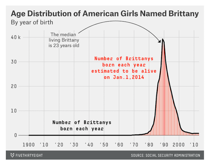
The most interesting analysis in the whole book comes when the name Leslie changes from male to female. There are many more fun things to discover. Five thirty eight ran a fun story on names a few years back with many more interesting charts. See this one for the name ‘Brittany’:

 

USDA Food Database

An entire chunk of code is missing from the book. It made it into the online Jupyter notebooks but I guess it was forgotten from the actual book.

# Missing code from book
>>> nutrients = []
>>> for rec in db:
        fnuts = pd.DataFrame(rec[‘nutrients’])
        fnuts[‘id’] = rec[‘id’]
        nutrients.append(fnuts)

>>> nutrients = pd.concat(nutrients, ignore_index=True)

PDA uses a convoluted way to find the food with the most nutrients:

>>> by_nutrient = ndata.groupby([‘nutgroup’, ‘nutrient’])
>>> get_maximum = lambda x: x.loc[x.value.idxmax()]
>>> max_foods = by_nutrient.apply(get_maximum)[[‘value’, ‘food’]]

A more clever approach involves sorting the column we want the maximum for ( value in this case) and then dropping all rows other than the first in the group with drop_duplicates. You must use the subset parameter here:

>>> max_foods = ndata.sort_values(‘value’, ascending=False) \
                     .drop_duplicates(subset=[‘nutrient’])

2012 Federal Election Commission Database

This should have been 2016 data since the book was published a year after the 2016 election.

The unstack method should be used with the fill_value parameter to fill in 0’s wherever there is missing data. It does not and instead returns NaNs.

Chapters 1–4 and the Appendices

Chapter 1 is a short chapter that gets you set up with Python and the scientific libraries. Chapters 2 and 3 quickly cover the basics of Python and the IPython command shell. These chapters will be of some help if you have no Python experience, but they won’t be enough on their own to prepare you for the material in the book.

The scope of PDA extends too far by covering basic Python and would have been better served to just omit it. Chapter 3 and the Appendix on NumPy are more helpful as pandas is built directly on top of it and the libraries are often intertwined together during a data analysis.

Conclusion: More Data Analysis and More Real Data

Python for Data Analysis teaches only the rudimentary mechanics on how to use a few of the pandas commands and does very little actual data analysis. If there is a third edition, I would suggest focusing on using real data sets with more advanced analysis.

Master Python, Data Science and Machine Learning

Immerse yourself in my comprehensive path for mastering data science and machine learning with Python. Purchase the All Access Pass to get lifetime access to all current and future courses. Some of the courses it contains:

• Exercise Python — A comprehensive introduction to Python (200+ pages, 100+ exercises)
• Master Data Analysis with Python — The most comprehensive course available to learn pandas. (600+ pages and 300+ exercises)
• Master Machine Learning with Python — A deep dive into doing machine learning with scikit-learn constantly updated to showcase the latest and greatest tools. (300+ pages)

Get the All Access Pass now!

Corporate Training

If you have a group at your company looking to learn directly from an expert who understands how to teach and motivate students, let me know by filling out the form on this page.